Introduction

In mathematics and statistics, random projection is a technique used to reduce the dimensionality of a set of points which lie in Euclidean space. Random projection methods are known for their simplicity and low error rates compared with other dimensionality-reduction techniques, and experiments show that they preserve pairwise distances well.

Consider a problem as follows: We have a set of $n$ points in a high-dimensional Euclidean space $\mathbf{R}^d$. We want to project the points onto a space of low dimension $\mathbf{R}^k$ in such a way that pairwise distances of the points are approximately the same as before.

Formally, we are looking for a map $f:\mathbf{R}^d\rightarrow\mathbf{R}^k$ such that for any pair of original points $u,v$, $\vert\vert f(u)-f(v)\vert\vert $ distorts little from $\vert\vert u-v\vert\vert $, where $\vert\vert \cdot\vert\vert $ is the Euclidean norm, i.e. $\vert\vert u-v\vert\vert =\sqrt{(u_1-v_1)^2+(u_2-v_2)^2+\ldots+(u_d-v_d)^2}$ is the distance between $u$ and $v$ in Euclidean space.

This problem has various important applications in both theory and practice. In many tasks, the data points are drawn from a high-dimensional space; however, computations on high-dimensional data are usually hard due to the infamous “curse of dimensionality”. The computational tasks can be greatly eased if we can project the data points onto a space of low dimension while the pairwise relations between the points are approximately preserved.

Johnson-Lindenstrauss Theorem

The Johnson-Lindenstrauss Theorem states that it is possible to project $n$ points in a space of arbitrarily high dimension onto an $O(\log n)$-dimensional space, such that the pairwise distances between the points are approximately preserved.

For any $0 < \epsilon < 1$ and any positive integer $n$, let $k$ be a positive integer such that

$$k\ge4(\epsilon^2/2-\epsilon^3/3)^{-1}\ln n$$

Then for any set $V$ of $n$ points in $\mathbf{R}^d$, there is a map $f:\mathbf{R}^d\rightarrow\mathbf{R}^k$ such that for all $u,v\in V$,

$$(1-\epsilon)\vert\vert u-v\vert\vert ^2\le\vert\vert f(u)-f(v)\vert\vert ^2\le(1+\epsilon)\vert\vert u-v\vert\vert ^2$$

Furthermore, this map can be found in expected polynomial time.

The Random Projections

The map $f:\mathbf{R}^d\rightarrow\mathbf{R}^k$ is done by random projection. There are several ways of applying the random projection. We adopt the one in the original Johnson-Lindenstrauss paper.

Let $A$ be a random $k\times d$ matrix that projects $\mathbf{R}^d$ onto a uniform random $k$-dimensional subspace.

Multiply $A$ by a fixed scalar $\sqrt{\frac{d}{k}}$. For every $v\in\mathbf{R}^d$, $v$ is mapped to $\sqrt{\frac{d}{k}}Av$.

The projected point $\sqrt{\frac{d}{k}}Av$ is a vector in $\mathbf{R}^k$.

The purpose of multiplying the scalar $\sqrt{\frac{d}{k}}$ is to guarantee that $\mathbf{E}\left[\left\vert\vert \sqrt{\frac{d}{k}}Av\right\vert\vert ^2\right]=\vert\vert v\vert\vert ^2$.

Besides the uniform random subspace, there are other choices of random projections known to have good performance, including:

• A matrix whose entries follow i.i.d. Gaussian distributions $N(0, \frac{1}{k})$.
• A matrix based on i.i.d. sampling described by:
  $w_{i, j} = \sqrt{s}\begin{cases}1 & \text{with prob. }\frac{1}{2s} \\0 & \text{with prob. }1-\frac{1}{s} \\-1 & \text{with prob. }\frac{1}{2s} \end{cases}$
  where $s$ is set to $\sqrt{d}$.

In both cases, the matrix is also multiplied by a fixed scalar for normalization.

A Proof of the Theorem

We present a proof due to Dasgupta-Gupta, which is much simpler than the original proof of Johnson-Lindenstrauss. The proof is for the projection onto uniform random subspace. The idea of the proof is outlined as follows:

1. To bound the distortions to pairwise distances, it is sufficient to bound the distortions to the length of unit vectors.
2. A uniform random subspace of a fixed unit vector is identically distributed as a fixed subspace of a uniform random unit vector. We can fix the subspace as the first $k$ coordinates of the vector, thus it is sufficient to bound the length (norm) of the first $k$ coordinates of a uniform random unit vector.
3. Prove that for a uniform random unit vector, the length of its first $k$ coordinates is concentrated to the expectation.

From pairwise distances to norms of unit vectors

Let $w\in \mathbf{R}^d$ be a vector in the original space. The random $k\times d$ matrix $A$ projects $w$ onto a uniformly random $k$-dimensional subspace of $\mathbf{R}^d$. We only need to show that

$$ \Pr\left[\left\vert\vert \sqrt{\frac{d}{k}}Aw\right\vert\vert ^2<(1-\epsilon)\vert\vert w\vert\vert ^2\right]\le\frac{1}{n^2}; $$

and

$$ \Pr\left[\left\vert\vert \sqrt{\frac{d}{k}}Aw\right\vert\vert ^2>(1+\epsilon)\vert\vert w\vert\vert ^2\right]\le\frac{1}{n^2}. $$

Think of $w$ as $w = u - v$ for some $u,v\in V$. Then by applying the union bound to all ${n\choose 2}$ pairs of the $n$ points in $V$, the random projection $A$ violates the distortion requirement with probability at most

$${n\choose 2}\cdot\frac{2}{n^2}=1-\frac{1}{n}$$

so $A$ has the desirable low-distortion with probability at least $\frac{1}{n}$. Thus, the low-distortion embedding can be found by trying for expected $n$ times (recalling the analysis of geometric distribution).

We can further simplify the problem by normalizing $w$. Note that for nonzero $w$’s, the statement that

$$(1-\epsilon)\vert\vert w\vert\vert ^2\le\left\vert\vert \sqrt{\frac{d}{k}}Aw\right\vert\vert ^2\le(1+\epsilon)\vert\vert w\vert\vert ^2$$

is equivalent to that

$$(1-\epsilon)\frac{k}{d}\le\left\vert\vert A\left(\frac{w}{\vert\vert w\vert\vert }\right)\right\vert\vert ^2\le(1+\epsilon)\frac{k}{d}$$

Thus, we only need to bound the distortions for the unit vectors, i.e. the vectors $w\in\mathbf{R}^d$ that $\vert\vert w\vert\vert =1$. The rest of the proof is to prove the following lemma for the unit vector in $\mathbf{R}^d$.

Lemma 1

For any unit vector $w\in\mathbf{R}^d$, it holds that

$$ \Pr\left[\vert\vert Aw\vert\vert ^2<(1-\epsilon)\frac{k}{d}\right]\le \frac{1}{n^2} $$$$ \Pr\left[\vert\vert Aw\vert\vert ^2>(1+\epsilon)\frac{k}{d}\right]\le \frac{1}{n^2} $$

As we argued above, this lemma implies the Johnson-Lindenstrauss theorem.

Random projection of fixed unit vector $\equiv$ fixed projection of random unit vector

Let $w\in\mathbf{R}^d$ be a fixed unit vector in $\mathbf{R}^d$. Let $A$ be a random matrix which projects the points in $\mathbf{R}^d$ onto a uniformly random $k$-dimensional subspace of $\mathbf{R}^d$.

Let $Y\in\mathbf{R}^d$ be a uniformly random unit vector in $\mathbf{R}^d$. Let $B$ be such a fixed matrix which extracts the first $k$ coordinates of the vectors in $\mathbf{R}^d$, i.e. for any $Y=(Y_1,Y_2,\ldots,Y_d)$, $BY=(Y_1,Y_2,\ldots, Y_k)$.

In other words, $Aw$ is a random projection of a fixed unit vector; and $BY$ is a fixed projection of a uniformly random unit vector. A key observation is that:

The distribution of $\vert\vert Aw\vert\vert $ is the same as the distribution of $\vert\vert BY\vert\vert $.

The proof of this observation is omitted here.

With this observation, it is sufficient to work on the subspace of the first $k$ coordinates of the uniformly random unit vector $Y\in\mathbf{R}^d$. Our task is now reduced to the following lemma.

Lemma 2

Let $Y=(Y_1,Y_2,\ldots,Y_d)$ be a uniformly random unit vector in $\mathbf{R}^d$. Let $Z=(Y_1,Y_2,\ldots,Y_k)$ be the projection of $Y$ to the subspace of the first $k$ coordinates of $\mathbf{R}^d$.

Then

$$\Pr\left[\vert\vert Z\vert\vert ^2<(1-\epsilon)\frac{k}{d}\right]\le \frac{1}{n^2}$$$$\Pr\left[\vert\vert Z\vert\vert ^2>(1+\epsilon)\frac{k}{d}\right]\le \frac{1}{n^2}$$

Due to the above observation, Lemma 2 implies Lemma 1 and thus proves the Johnson-Lindenstrauss theorem.

Note that $\vert\vert Z\vert\vert ^2=\sum_{i=1}^kY_i^2$. Due to the linearity of expectations,

$$\mathbf{E}[\vert\vert Z\vert\vert ^2]=\sum_{i=1}^k\mathbf{E}[Y_i^2].$$

Since $Y$ is a uniform random unit vector, it holds that $\sum_{i=1}^dY_i^2=\vert\vert Y\vert\vert ^2=1$. And due to the symmetry, all $\mathbf{E}[Y_i^2]$’s are equal. Thus, $\mathbf{E}[Y_i^2]=\frac{1}{d}$ for all $i$. Therefore, $\mathbf{E}[\vert\vert Z\vert\vert ^2]=\sum_{i=1}^k\mathbf{E}[Y_i^2]=\frac{k}{d}$.

Lemma 2 actually states that $\vert\vert Z\vert\vert ^2$ is well-concentrated to its expectation.

Concentration of the norm of the first $k$ entries of uniform random unit vector

We now prove Lemma 2. Specifically, we will prove the $(1-\epsilon)$ direction:

$$\Pr[\vert\vert Z\vert\vert ^2<(1-\epsilon)\frac{k}{d}]\le\frac{1}{n^2}.$$

The $(1+\epsilon)$ direction is proved with the same argument.

Due to the discussion in the last section, this can be interpreted as a concentration bound for $\vert\vert Z\vert\vert ^2$, which is a sum of $Y_1^2,Y_2^2,\ldots,Y_k^2$. This suggests using Chernoff-like bounds. However, for a uniformly random unit vector $Y$, the $Y_i$’s are not independent (because of the constraint that $\vert\vert Y\vert\vert =1$). We overcome this by generating uniform unit vectors from independent normal distributions.

The following is a very useful fact regarding the generation of uniform unit vectors.

Let $X_1,X_2,\ldots,X_d$ be i.i.d. random variables, each drawn from the normal distribution $N(0,1)$. Let $X=(X_1,X_2,\ldots,X_d)$. Then

$$Y=\frac{1}{\vert\vert X\vert\vert }X$$

is a uniformly random unit vector.

Then for $Z=(Y_1,Y_2,\ldots,Y_k)$, $\vert\vert Z\vert\vert ^2=Y_1^2+Y_2^2+\cdots+Y_k^2=\frac{X_1^2}{\vert\vert X\vert\vert ^2}+\frac{X_2^2}{\vert\vert X\vert\vert ^2}+\cdots+\frac{X_k^2}{\vert\vert X\vert\vert ^2}=\frac{X_1^2+X_2^2+\cdots+X_k^2}{X_1^2+X_2^2+\cdots+X_d^2}$.

To avoid writing a lot of $(1-\epsilon)$’s, we write $\beta = (1-\epsilon)$. The first inequality (the lower tail) of Lemma 2 can be written as:

$$ \begin{align}\Pr\left[\vert\vert Z\vert\vert ^2<\frac{\beta k}{d}\right] &=\Pr\left[\frac{X_1^2+X_2^2+\cdots+X_k^2}{X_1^2+X_2^2+\cdots+X_d^2}<\frac{\beta k}{d}\right]\\ &=\Pr\left[d(X_1^2+X_2^2+\cdots+X_k^2)<\beta k(X_1^2+X_2^2+\cdots+X_d^2)\right]\\ &=\Pr\left[(\beta k-d)\sum_{i=1}^k X_i^2+\beta k\sum_{i=k+1}^d X_i^2>0\right]. &\qquad (**) \end{align} $$

The probability is a tail probability of the sum of $d$ independent variables. The $X_i^2$’s are not 0-1 variables, thus we cannot directly apply the Chernoff bounds. However, the following two key ingredients of the Chernoff bounds hold for the above sum:

• The $X_i^2$’s are independent.
• Because $X_i^2$’s are normal, it is known that the moment generating functions for $X_i^2$’s can be computed as follows:
  Fact 1
  If $X$ follows the normal distribution $N(0,1)$, then $\mathbf{E}\left[e^{\lambda X^2}\right]=(1-2\lambda)^{-\frac{1}{2}}$, for $\lambda\in\left(-\infty,1/2\right)$.

Therefore, we can re-apply the technique of the Chernoff bound (applying Markov’s inequality to the moment generating function and optimizing the parameter $\lambda$) to bound the probability ( ** ):

$$ \begin{align} &\Pr\left[(\beta k-d)\sum_{i=1}^k X_i^2+\beta k\sum_{i=k+1}^d X_i^2>0\right]\\ &=\Pr\left[\exp\left\{(\beta k-d)\sum_{i=1}^k X_i^2+\beta k\sum_{i=k+1}^d X_i^2\right\}>1\right] \\ &=\Pr\left[\exp\left\{\lambda\left((\beta k-d)\sum_{i=1}^k X_i^2+\beta k\sum_{i=k+1}^d X_i^2\right)\right\}>1\right] &\quad (\text{for }\lambda>0) \\ &\le \mathbf{E}\left[\exp\left\{\lambda\left((\beta k-d)\sum_{i=1}^k X_i^2+\beta k\sum_{i=k+1}^d X_i^2\right)\right\}\right] &\quad \text{(by Markov inequality)} \\ &= \prod_{i=1}^k\mathbf{E}\left[e^{\lambda(\beta k-d)X_i^2}\right]\cdot\prod_{i=k+1}^d\mathbf{E}\left[e^{\lambda\beta k X_i^2}\right] &\quad (\text{independence of }X_i) \\ &= \mathbf{E}\left[e^{\lambda(\beta k-d)X_1^2}\right]^{k}\cdot\mathbf{E}\left[e^{\lambda\beta k X_1^2}\right]^{d-k}&\quad \text{(symmetry)} \\ &=(1-2\lambda(\beta k-d))^{-\frac{k}{2}}(1-2\lambda\beta k)^{-\frac{d-k}{2}}&\quad \text{(by Fact 1)} \end{align} $$

The last term $(1-2\lambda(\beta k-d))^{-\frac{k}{2}}(1-2\lambda\beta k)^{-\frac{d-k}{2}}$ is minimized when $\lambda=\frac{1-\beta}{2\beta(d-k\beta)}$, so that

$$ \begin{align} &(1-2\lambda(\beta k-d))^{-\frac{k}{2}}(1-2\lambda\beta k)^{-\frac{d-k}{2}} \\ &=\beta^{\frac{k}{2}}\left(1+\frac{(1-\beta)k}{(d-k)}\right)^{\frac{d-k}{2}} \\ &\le \exp\left(\frac{k}{2}(1-\beta+\ln \beta)\right) &\qquad (\text{since }\left(1+\frac{(1-\beta)k}{(d-k)}\right)^{\frac{d-k}{(1-\beta)k}}\le e) \\ &= \exp\left(\frac{k}{2}(\epsilon+\ln (1-\epsilon))\right)&\qquad (\beta=1-\epsilon)\\&\le\exp\left(-\frac{k\epsilon^2}{4}\right) &\qquad (\text{by Taylor expansion }\ln(1-\epsilon)\le-\epsilon-\frac{\epsilon^2}{2}) \end{align} $$

which is $\le\frac{1}{n^2}$ for the choice of $k$ in the Johnson-Lindenstrauss theorem that $k\ge4(\epsilon^2/2-\epsilon^3/3)^{-1}\ln n$.

So we have proved that

$$\Pr[\vert\vert Z\vert\vert ^2<(1-\epsilon)\frac{k}{d}]\le\frac{1}{n^2}.$$

With the same argument, the other direction can be proved so that

$$\Pr[\vert\vert Z\vert\vert ^2>(1+\epsilon)\frac{k}{d}]\le \exp\left(\frac{k}{2}(-\epsilon+\ln (1+\epsilon))\right)\le\exp\left(-\frac{k(\epsilon^2/2-\epsilon^3/3)}{2}\right)$$

which is also $\le\frac{1}{n^2}$ for $k\ge4(\epsilon^2/2-\epsilon^3/3)^{-1}\ln n$.

Lemma 2 is proved. As we discussed in the previous sections, Lemma 2 implies Lemma 1, which implies the Johnson-Lindenstrauss theorem.

Experiments

Minimal Size of the Random Subspace

Knowing only the number of samples, we can conservatively estimate the minimal size of the random subspace according to the Johnson-Lindenstrauss lemma to guarantee a bounded distortion introduced by the random projection:

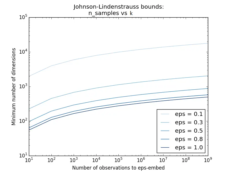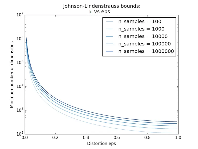The left plot shows that the minimal dimension $k$ grows only logarithmically with the number of samples $n$ (and does not depend on the original dimension $d$ at all), while the right plot shows that $k$ blows up rapidly as the allowed distortion $\epsilon$ approaches $0$. This is why random projection stays practical even for very large datasets, as long as a moderate distortion is acceptable.

Gaussian Random Projection

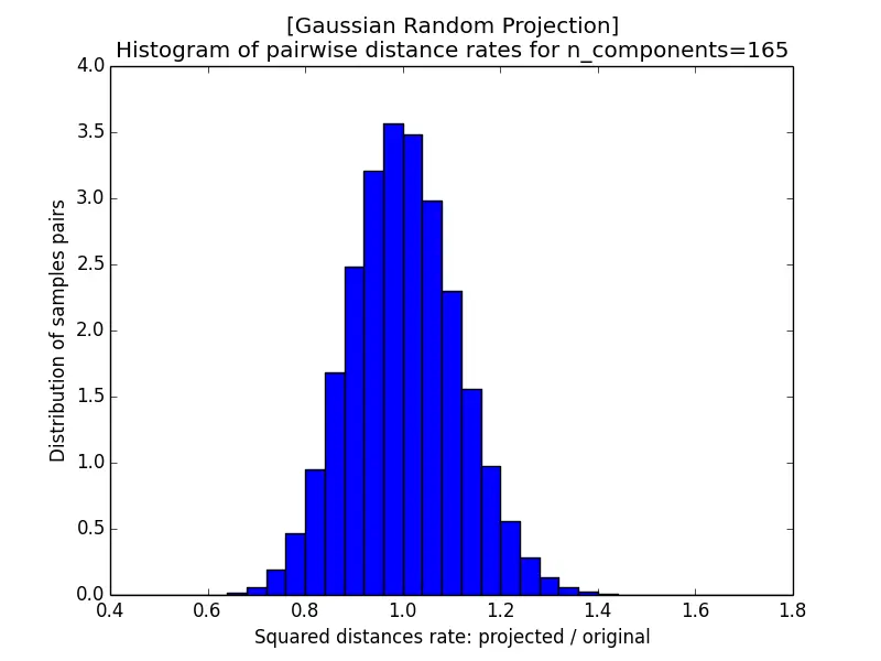
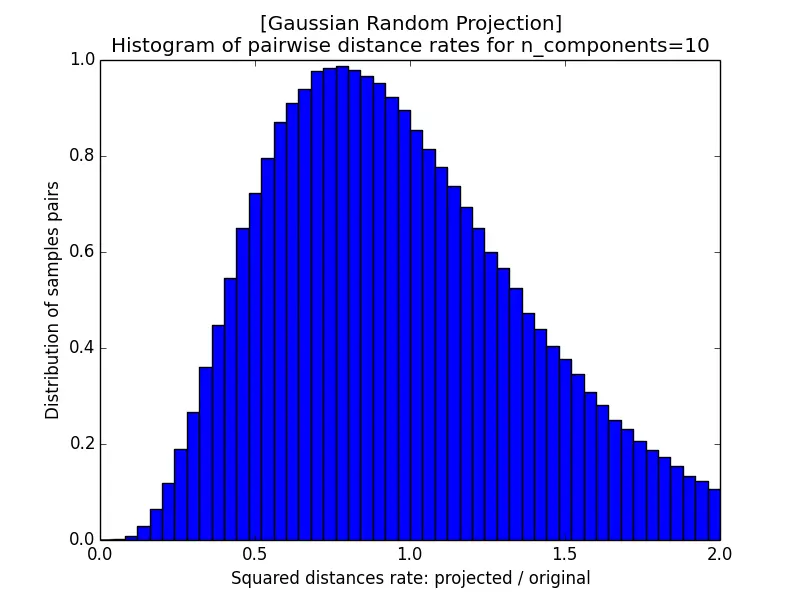
In the following subsections, we project a matrix $\mathbf{A}$ of dimension $1000 \times 100000$ (i.e. $n = 1000$ points in $d = 100000$ dimensions) onto a subspace $\widehat{\mathbf{A}}_{1000 \times k}$, where $k \in \left\{5920, 332, 165, 10\right\}$. By the Johnson-Lindenstrauss bound $k\ge4(\epsilon^2/2-\epsilon^3/3)^{-1}\ln n$ with $n = 1000$, these target dimensions correspond to a maximum distortion rate (as defined by the lemma) of roughly $\epsilon \approx 0.1, 0.5, 0.9$, and (for $k = 10$) a value larger than $1$ for which the lemma offers no guarantee.

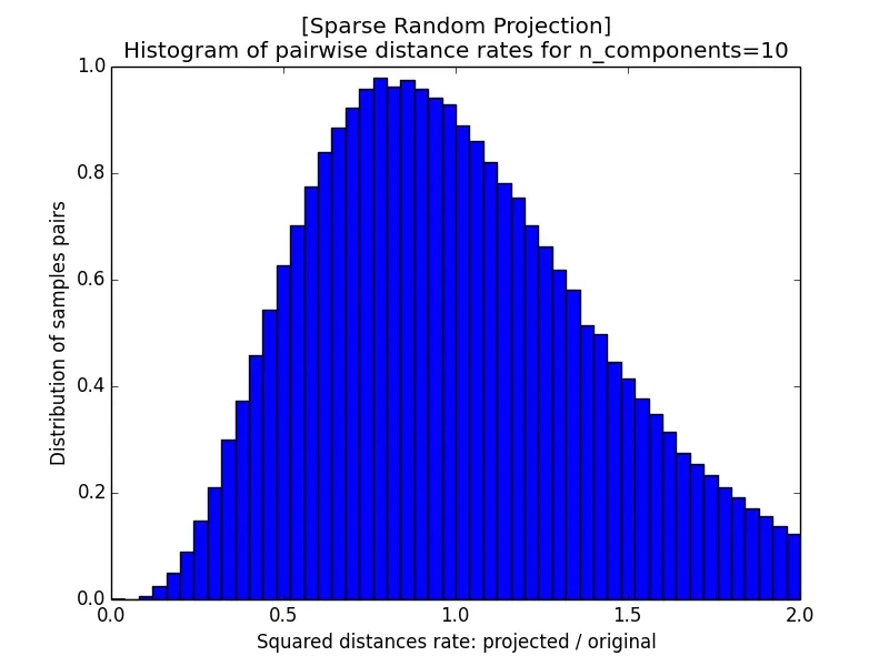
The images below show the histogram of pairwise distance rates (the ratio of the squared distance after projection to the squared distance before projection) for different $\epsilon$; a perfectly distance-preserving projection would put all the mass at a rate of $1$. With $k = 5920$ the rates are tightly concentrated within $[0.95, 1.05]$, but as $k$ shrinks the histogram widens, and at $k = 10$ it spreads all the way from near $0$ to $2$. A smaller $\epsilon$, which requires a larger target dimension $k$, therefore yields better-preserved distances.

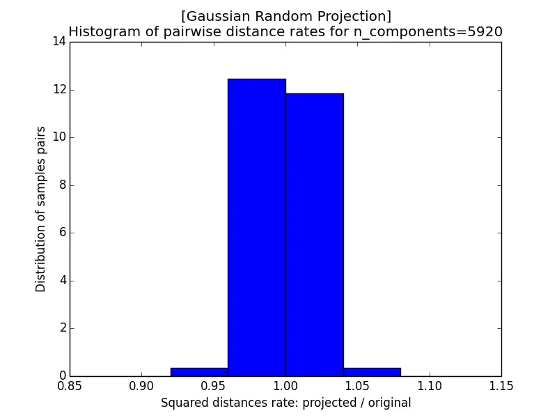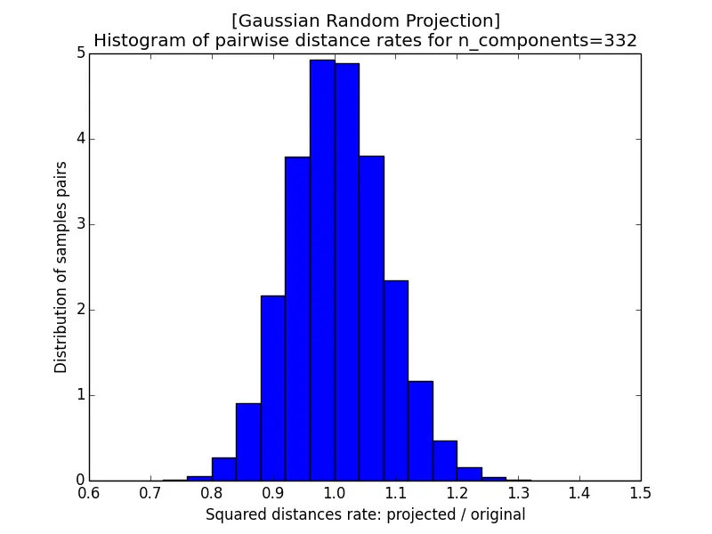a) k=5920	b) k=332
c) k=165	d) k=10

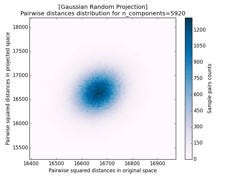
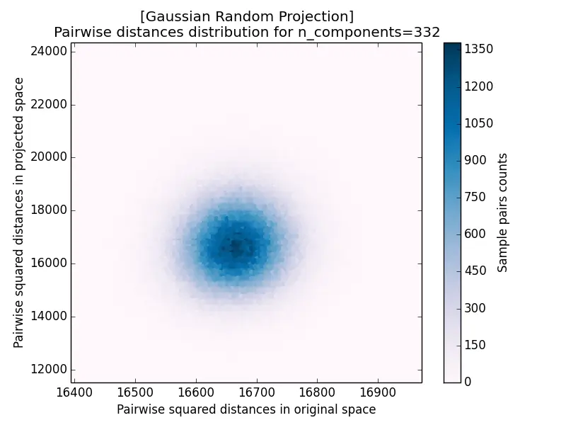
Another measurement for projection results is the pairwise distance distribution, which plots the squared distance of each pair after projection against its squared distance before projection. The closer the cloud hugs the diagonal, the better distances are preserved: it forms a tight blob centered on the diagonal for $k = 5920$ and disperses increasingly as $k$ decreases.

a) k=5920	b) k=332
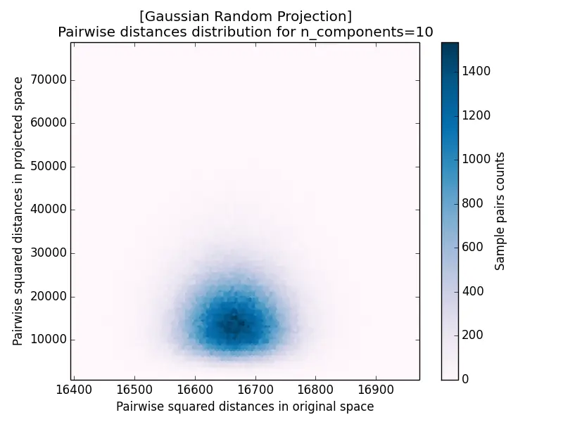c) k=165	d) k=10

Sparse Random Projection

Sparse Random Projection (with $s = 3$) produces almost the same distance-rate histograms as the Gaussian case, while using a much sparser projection matrix that is cheaper to store and faster to multiply.

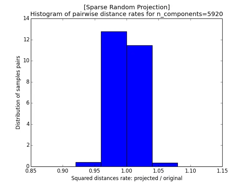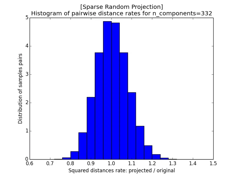a) k=5920	b) k=332
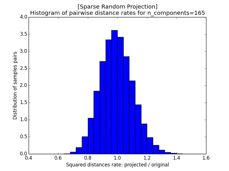c) k=165	d) k=10

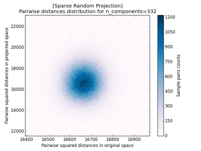
The distance distribution for Sparse Random Projection is shown below, and it again matches the Gaussian case closely: a tight cluster on the diagonal for large $k$ that spreads out as $k$ decreases.

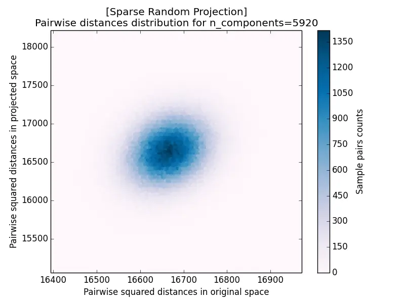a) k=5920	b) k=332
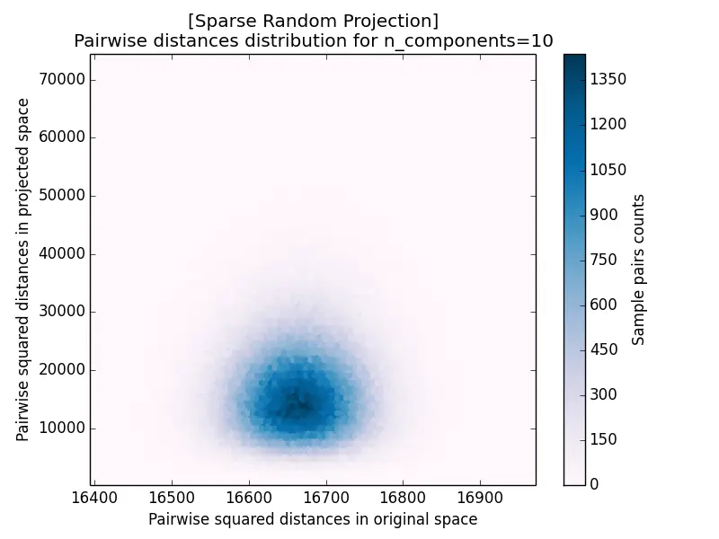c) k=165	d) k=10

Conclusion

Random projection is a popular technique for dimensionality reduction because of its high computational efficiency. There are two ways to generate random matrices for projection: a Gaussian matrix or a sparse matrix. For $s = 3$ in Sparse Random Projection, the results for Gaussian Random Projection and Sparse Random Projection are almost the same. Another thing to consider in random projection is the target dimensionality $k$: a larger $k$ (equivalently, a smaller distortion bound $\epsilon$) results in better projection accuracy but takes longer.

Reference

• Random projection (Wikipedia)
• 随机算法 (Fall 2011) / Johnson-Lindenstrauss Theorem (Nanjing University TCS Wiki)
• Random Projection (scikit-learn documentation)