AdaBoost
AdaBoost, short for “Adaptive Boosting”, is a machine learning meta-algorithm formulated by Yoav Freund and Robert Schapire who won the Gödel Prize in 2003 for their work. The output of the other learning algorithms (weak learners) is combined into a weighted sum that represents the final output of the boosted classifier.
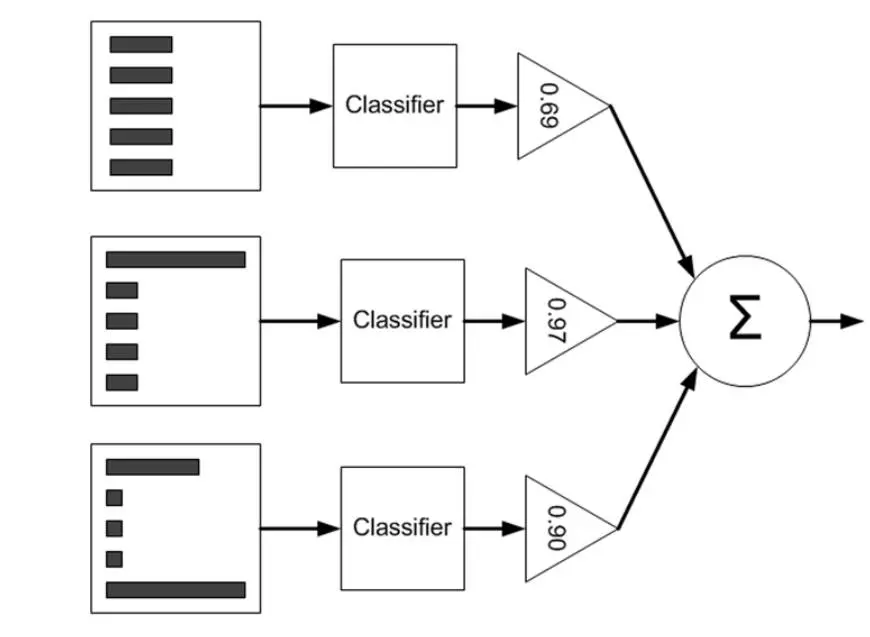
AdaBoost is adaptive in the sense that subsequent weak learners are tweaked in favor of those instances misclassified by previous classifiers. AdaBoost is sensitive to noisy data and outliers and is quite robust to overfitting.
Bagging vs. Boosting
A too complex model (unpruned decision trees) has high variance but low bias, whereas a too simple model (weak learners like decision stumps) has high bias but low variance. To minimize these two types of errors two different approaches are required namely bagging (complex models/high variance) and boosting (simple models/high bias).
- Bagging (stands for Bootstrap Aggregation) is the way to decrease the variance of your prediction by generating additional data for training from your original dataset using combinations with repetitions to produce multisets of the same cardinality/size as your original data. By increasing the size of your training set you can’t improve the model predictive force, but just decrease the variance, narrowly tuning the prediction to expected outcome. Random Forest is a typical example of bagging.
- Boosting is a two-step approach, where one first uses subsets of the original data to produce a series of averagely performing models and then “boosts” their performance by combining them together using a particular cost function (=majority vote). Unlike bagging, in the classical boosting the subset creation is not random and depends upon the performance of the previous models: every new subset contains the elements that were (likely to be) misclassified by previous models. Adaboost is a typical example of boosting.
AdaBoost Algorithm
Given a training set with two classes:
$$\mathbf{T}=\left\{(\mathbf{x}_1, y_1), (\mathbf{x}_2, y_2), \dots, (\mathbf{x}_N, y_N)\right\}$$where $\mathbf{x}_i \in \mathbb{R}^d$ and $y_i \in \left\{-1, +1\right\}$. The procedure of AdaBoost can be described as follows:
Input: training set $\mathbf{T}$
Output: the final classifier $G(x)$.
- Initialize weights of training examples: $$\begin{align}\mathbf{D}_1 = (w_{11}, \dots, w_{1i}, \dots, w_{1N}), w_{1i} = \frac{1}{N}, i = 1, 2, \dots, N\end{align}$$
- For $m = 1, 2, \dots, M$ (where $M$ is the number of weak classifiers)
- Fit a classifier $G_m(x)$ to the training data using weights $w_{mi}$
- Compute misclassification error of $G_m(x)$:
$$\begin{align}e_m = P(G_m(\mathbf{x}_i)\ne y_i) =\sum_{i=1}^{N}{w_{mi} I(G_m(\mathbf{x}_i) \ne y_i)}\end{align}$$ - Compute the weight $\alpha_m$ for this classifier $G_m(x)$ $$\begin{align}\alpha_m = \frac{1}{2}\ln\frac{1 - e_m}{e_m}\end{align}$$
- Update weights of training examples:
$$\begin{align}\mathbf{D}_{m+1} = (w_{m+1, 1}, \dots, w_{m+1, i}, \dots, w_{m+1, N})\end{align}$$ $$\begin{align}w_{m+1, i} = \frac{w_{m, i}}{Z_m} \exp(-\alpha_m y_i G_m(\mathbf{x}_i))\end{align}$$ where $Z_m = \sum_{i=1}^{N}{w_{mi}\exp(-\alpha_m y_i G_m(\mathbf{x}_i))}$ is a normalization factor that makes $\mathbf{D}_{m+1}$ sum to 1.
- The final classifier $G(x)$ is the weighted sum of each iteration’s classifier output $G_m(x)$, weighted by $\alpha_m$. $$\begin{align}G(x) = \text{sign}(f(x)) = \text{sign}\left(\sum_{m=1}^{M}{\alpha_m G_m(x)}\right)\end{align}$$
$\alpha_m$ stands for the weight of the $m$-th classifier. From the formula for $\alpha_m$ above, $\alpha_m \ge 0$ when $e_m \le \frac{1}{2}$, and $\alpha_m$ increases as $e_m$ decreases. Therefore, the classifiers with lower classification error have higher weights in the final classifier.
Example of AdaBoost
The training examples are given below:
| $x$ | 0 | 1 | 2 | 3 | 4 | 5 | 6 | 7 | 8 | 9 |
|---|---|---|---|---|---|---|---|---|---|---|
| $y$ | 1 | 1 | 1 | -1 | -1 | -1 | 1 | 1 | 1 | -1 |
- Initialize weights of training examples:
$\mathbf{D}_1=(w_{11}, w_{12}, \dots, w_{1,10})$
$w_{1i} = \frac{1}{10}, i = 1, 2, \dots, 10$ - For $m = 1$:
- The misclassification error of the classifier $G_1(\mathbf{x})$ has the minimum value when $v = 2.5$ in training examples with weights $\mathbf{D}_1$
$G_1(\mathbf{x}) = \begin{cases}1, & x<2.5\\-1, & x\ge2.5\end{cases}$ - The misclassification error of $G_1(\mathbf{x})$: $e_1=P(G_1(\mathbf{x}_i) \ne y_i)=0.3$
- Compute the weight of the classifier $G_1$: $\alpha_1 = \frac{1}{2} \ln\frac{1 - e_1}{e_1}=0.4236$
- Update the weight of training examples:
$D_2 = (w_{21}, \dots, w_{2i}, \dots, w_{2,10})$
$w_{2i} = \frac{w_{1i}}{Z_1} \exp(-\alpha_1 y_i G_1(x_i)), i = 1, 2, \dots, 10$
$D_2 = (0.0714, 0.0714, 0.0714, 0.0714, 0.0714, 0.0714, 0.1667, 0.1667, 0.1667, 0.0714)$
$f_1(\mathbf{x}) = 0.4236G_1(\mathbf{x})$ - There are 3 examples misclassified by the classifier: $\text{sign}[f_1(\mathbf{x})]$.
- The misclassification error of the classifier $G_1(\mathbf{x})$ has the minimum value when $v = 2.5$ in training examples with weights $\mathbf{D}_1$
- For $m = 2$:
- The misclassification error of the classifier $G_2(\mathbf{x})$ has the minimum value when $v = 8.5$ in training examples with weights $\mathbf{D}_2$
$G_2(\mathbf{x}) = \begin{cases}1, & x<8.5\\-1, & x\ge8.5\end{cases}$ - The misclassification error of $G_2(\mathbf{x})$: $e_2=0.2143$
- Compute the weight of the classifier $G_2$: $\alpha_2 = \frac{1}{2} \ln\frac{1 - e_2}{e_2}=0.6496$
- Update the weight of training examples:
$D_3 = (0.0455, 0.0455, 0.0455, 0.1667, 0.1667, 0.1667, 0.1060, 0.1060, 0.1060, 0.0455)$
$f_2(\mathbf{x}) = 0.4236G_1(\mathbf{x}) + 0.6496G_2(\mathbf{x})$ - There are 3 examples misclassified by the classifier: $\text{sign}[f_2(\mathbf{x})]$.
- The misclassification error of the classifier $G_2(\mathbf{x})$ has the minimum value when $v = 8.5$ in training examples with weights $\mathbf{D}_2$
- For $m = 3$:
- The misclassification error of the classifier $G_3(\mathbf{x})$ has the minimum value when $v = 5.5$ in training examples with weights $\mathbf{D}_3$
$G_3(\mathbf{x}) = \begin{cases}1, & x<5.5\\-1, & x\ge5.5\end{cases}$ - The misclassification error of $G_3(\mathbf{x})$: $e_3=0.1820$
- Compute the weight of the classifier $G_3$: $\alpha_3 = \frac{1}{2} \ln\frac{1 - e_3}{e_3}=0.7514$
- Update the weight of training examples:
$D_4 = (0.125, 0.125, 0.125, 0.102, 0.102, 0.102, 0.065, 0.065, 0.065, 0.125)$
$f_3(\mathbf{x}) = 0.4236G_1(\mathbf{x}) + 0.6496G_2(\mathbf{x}) + 0.7514G_3(\mathbf{x})$ - All examples can be classified correctly by the classifier: $\text{sign}[f_3(\mathbf{x})]$.
- The misclassification error of the classifier $G_3(\mathbf{x})$ has the minimum value when $v = 5.5$ in training examples with weights $\mathbf{D}_3$
- The final classifier is $G(\mathbf{x}) = \text{sign}[f_3(\mathbf{x})] = \text{sign}[0.4236G_1(\mathbf{x}) + 0.6496G_2(\mathbf{x}) + 0.7514G_3(\mathbf{x})]$
AdaBoost and Forward Stagewise Modeling
So far we have simply stated the formula $\alpha_m = \frac{1}{2}\ln\frac{1 - e_m}{e_m}$ without justifying it. This section shows that AdaBoost is in fact a forward stagewise procedure that greedily minimizes an exponential loss, and that this minimization is exactly where the formula for $\alpha_m$ comes from.
Forward Stagewise Modeling
An additive model can be formulated as follows:
$$ f(x) = \sum_{m=1}^{M} \beta_m b(x; \gamma_m) $$where $b(x; \gamma_m)$ are the basis functions, $\gamma_m$ and $\beta_m$ are the parameters and weights of the basis functions respectively.
Additive models are fit by minimizing a loss function $L(y, f(x))$ averaged over the training data:
$$ \min_{\{\beta_m, \gamma_m\}_{m=1}^M} \sum_{i=1}^{N} L \left( y_i, \sum_{m=1}^M \beta_m b(x_i; \gamma_m) \right) $$Directly optimizing such loss function is often difficult. However, if optimizing over one single base function
$$ \min_{\{\beta, \gamma\}} \sum_{i=1}^{N} L \left( y_i, \beta b(x_i; \gamma) \right) $$can be done efficiently, a simple greedy search method can be used. The basic idea is to sequentially add new base functions to the expansion function $f(x)$ without changing the parameters that have been added.
The procedure of forward stagewise algorithm is listed below:
Input: Training set $T = \{(x_1, y_1), (x_2, y_2), \dots, (x_N, y_N)\}$; Loss function: $L(y, f(x))$; basis functions set: $\{b(x; \gamma)\}$
Output: Additive model $f(x)$
- Initialize $f_0(x) = 0$
- For $m = 1, 2, \dots, M$
- Minimize the loss function
$$\begin{align} (\beta_m, \gamma_m) = \operatorname*{arg\,min}_{\beta, \gamma} \sum_{i = 1}^{N} L \left( y_i, f_{m-1}(x_i) + \beta b(x_i; \gamma) \right)\end{align}$$ - Update additive model
$$\begin{align}f_m(x) = f_{m - 1}(x) + \beta_m b(x; \gamma_m)\end{align}$$
- Minimize the loss function
- The additive model can be calculated as $$\begin{align}f(x) = f_M(x) = \sum_{m=1}^M \beta_m b(x; \gamma_m)\end{align}$$
AdaBoost Fits an Additive Model
AdaBoost fits an additive model by forward stagewise approach, where
- the base function $b_m$ is a binary classifier $G_m(x): \mathbb{R}^d \rightarrow \{-1, 1\}$;
- the objective function is the exponential loss: $L(y, f(x)) = \exp[-y f(x)]$
First we write down the exponential loss:
$$ (\alpha_m, G_m) = \operatorname*{arg\,min}_{\alpha, G} \sum_{i = 1}^{N} \exp \left(- y_i ( f_{m-1}(x_i) + \alpha G(x_i)) \right) $$Then define weights $\omega_i^{(m)} = \exp(- y_i f_{m-1}(x_i))$, and divide the training data into two subsets, $\{y_i = G(x_i)\}$ and $\{y_i \ne G(x_i)\}$:
$$ \begin{align} L(\alpha, G) &= \sum_{i=1}^N \exp[-y_i[f_{m-1}(x_i) + \alpha G(x_i)]] \\ &=\sum_{i=1}^N \omega_i^{(m)} \exp(-y_i \alpha G(x_i)) \\ &=e^{-\alpha}\sum_{y_i = G(x_i)} \omega_i^{(m)} + e^{\alpha}\sum_{y_i \ne G(x_i)} \omega_i^{(m)}\\ &=e^{-\alpha}\sum_{i=1}^N \omega_i^{(m)} + (e^{\alpha} - e^{-\alpha})\sum_{i=1}^N \omega_i^{(m)} I(y_i \ne G(x_i)) \end{align} $$Then we optimize this loss function over $\alpha$ and $G(x)$ iteratively. Once $\alpha$ is fixed, the optimal $G_m^*(x)$ is given by
$$ G_m^*(x) = \operatorname*{arg\,min}_G \sum_{i=1}^N \omega_i^{(m)} I(y_i \ne G(x_i)) $$In other words, the optimal $G_m^*(x)$ is the classifier that minimizes the weighted prediction error, where $\omega_i^{(m)}$ is viewed as a weight assigned to the $i$-th training data.
Given a fixed $G_m$, we substitute it into the loss function, take the derivative w.r.t. $\alpha_m$ and set it to zero.
$$ \frac{\partial L}{\partial \alpha_m} = \frac{\partial (e^{-\alpha}\sum_{y_i = G(x_i)} \omega_i^{(m)} + e^{\alpha}\sum_{y_i \ne G(x_i)} \omega_i^{(m)})}{\partial \alpha_m} = 0 $$that is
$$ \begin{align} \alpha_m^* &=\frac{1}{2} \ln \frac{1- e_m}{e_m} \\ e_m &= \frac{\sum_{i = 1}^N \omega_i^{(m)} I(y_i \ne G_m(x_i))}{\sum_{i=1}^N \omega_i^{(m)}} \end{align} $$Conclusion
The forward stagewise view ties everything together: in each round AdaBoost fits a weak classifier $G_m$ that minimizes the weighted error, then assigns it the weight $\alpha_m = \frac{1}{2}\ln\frac{1 - e_m}{e_m}$, the same closed-form update used in the algorithm above. The exponential weights $\omega_i^{(m)}$ are what make later learners concentrate on the examples that previous ones misclassified. This is why a sequence of weak learners, such as decision stumps, can be boosted into a single strong classifier.
References
- Hang Li. Statistical Learning Methods. Tsinghua University Press (2012)
- Freund, Yoav, and Robert E. Schapire. Experiments with a new boosting algorithm. ICML. Vol. 96. 1996.
- AdaBoost (Wikipedia)
- AdaBoost: Why It Is Robust to Overfitting (Vivek Mishra)
- Bagging, boosting and stacking in machine learning (Cross Validated)
- Boosting (10-701 recitation slides, CMU) \[PDF\]
The Disqus comment system is loading ...
If the message does not appear, please check your Disqus configuration.